Kim H. Esbensena and Claas Wagnerb
aKHE Consulting, www.kheconsult.com
bSampling Consultant—Specialist in Feed, Food and Fuel QA/QC. E-mail: [email protected]
Previous columns have been devoted to a comprehensive introduction to the basic principles, methods and equipment for sampling of stationary materials and lots, as part of a description of the systematics of the Theory of Sampling (TOS). The next instalment of columns will deal with process sampling, i.e. sampling from moving streams of matter. As will become clear there is a great deal of redundancy regarding how to sample both stationary and moving lots, but it is the specific issues pertaining to dynamic lots that will be highlighted.
Lot dimensionality: ease of practical sampling
The Theory of Sampling (TOS) has found it useful to classify lot geometry into four categories. The strict scientific definitions are not necessary at the introductory level in these columns, which will rather focus on lot dimensionality from the point of view of sampling efficiency (or sampling possibility, in difficult cases). A straightforward lot dimensionality classification is seen is Figure 1.
From a practical point of view, sampling needs to be concerned with the ease with which one is able to extract increments from a randomly chosen location in the lot (or selected according to a sampling plan). Thus it is relatively easy to extract slices of any lot which has one dimension which dominates, i.e. is vastly longer (the extension dimension) than any of the other two dimensions (width, height). From this sampling point of view, the lot is effectively only 1-dimensional because all material in an incremental slice “covers” completely the full width and height of the material. This is the reason for TOS’ classification of 1-dimensional lots, or 1-D bodies. 1-D lots have a special status in TOS, for various reasons (see further below). Observe that a 1-D lot can either be a stationary, very elongated body (stock, pile etc.) or it can be a dynamic 1-D lot, i.e. a moving or flowing stream of matter (the material being transported by a conveyor belt is an archetypal dynamic 1-D lot; likewise the moving matter confined to a pipeline). It is a very important issue that 1-D lot sampling increments have the form of a “slice”.
It is equally easy to define a 2-D body (see Figure 1). 2-dimensional lots are characterised by the fact that all increments will only “cover” one dimension. Very often 2-D lots are horizontal, with the remaining dimension vertical (think of a drill core penetrating a geological formation, or a layer), but not necessarily in this orientation. The defining issue is that there is only one degree of freedom, namely where in the X–Y plane is the 1-dimensional increment to be located “where to sample in the X–Y plane?”). The operative increments in sampling 2-D lots are either “cylindrical increments” or box-like, see Figure 1.
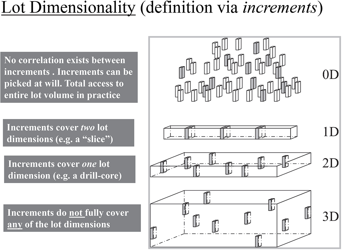
Figure 1. TOS’ practically oriented classification of lot dimensionality; the odd “0-dimensional lot” type is explained fully in the text. Illustration credit: Lars Petersen Julius (with permission).
The key feature for the sampler, or for the sampling equipment, is that there is full access to the entire lot in the case of 1-D and 2-D lots. This is an important empowerment because it allows the demands of the fundamental sampling principle (FSP) to be honoured: all potential increments from a lot must be accessible for physical extraction if/when selected. Indeed, this feature is scale-invariant, one can sample all 1,2-dimensional lots of any size under the FSP. Going on to 3-D lots leads to a perplexing revelation. It is very difficult to define a 3-D lot from the point of view of practical sampling, logically the operative increment form here should be a sphere. But in our 3-D world, extracting spherical increments is not exactly easy… … Be this as it may, TOS has many alternatives to offer for 3-D sampling, but this is outside the present scope (see, for example, Reference 1).
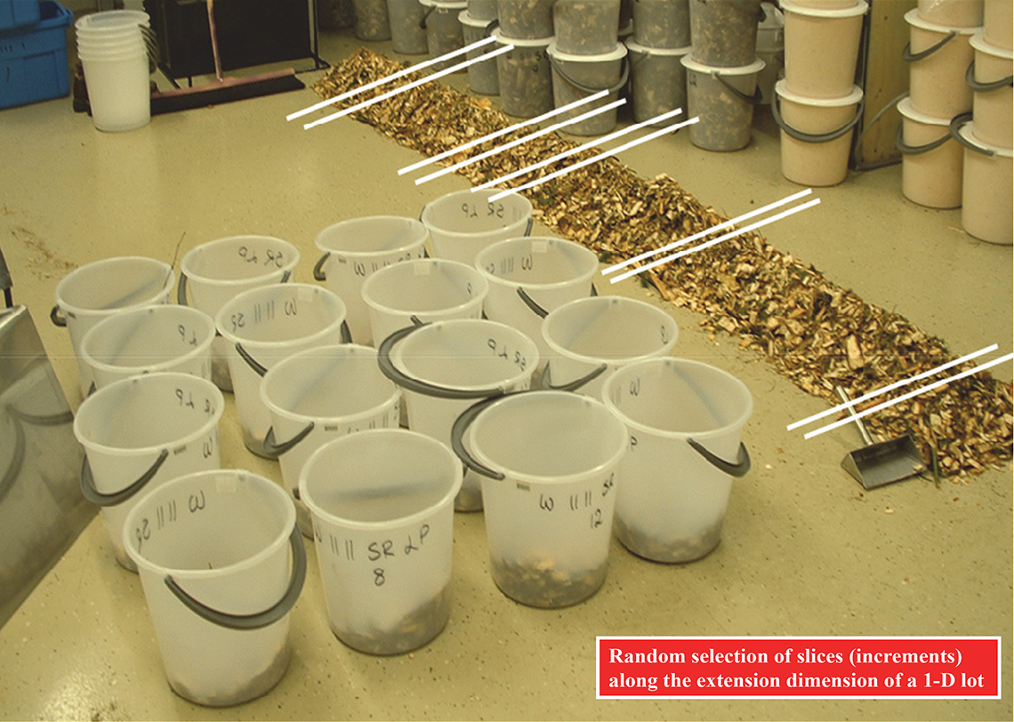
Figure 2. There should always be an element of randomness in a good sampling procedure, here the locations along the extension dimension of a 1-D lot are selected in this fashion. All slices correspond to complete slices of the width–height dimensions of the lot. Illustration credit: KHE.
WHAT then is a “0-dimensional lot”, the top illustration in Figure 1? This is another of TOS’ penetrating ways to focus on the underlying systematics of sampling. A 0-D lot is a lot that is “small” enough so that it is particularly easy always, under all circumstances, with all kinds of equipment to extract any size increment desired (increments of any form, so long as the increments are all congruent, i.e. of the exact same form and size). In other words, a 0-D lot is a particularly easy-to-sample lot. Obviously there is a grading demarcation between a 0-D lot and a 3-D lot, but in practice this discrimination has been found immensely useful. It is full accessibility in sampling practice that is the key operative element in these definitions.
Thus, with respect to sampling practice, lots come in groups [0-, 3-D lots] vs [1-, 2-D lots] of which the latter are of overwhelming importance—because this allows practical sampling no longer to be concerned with the size, magnitude, volume, mass of the lot. All [1-, 2-D lots] can be sampled appropriately, and this is a very large first step towards universal representativity.
Lot dimensionality transformation
This is a most advantageous feature of 1-D lot configurations. Irrespective of whether a 1-D lot is stationary or moving, it is 100% guaranteed that the entire lot will be available for increment extraction. 1-D lots are always particularly easy to sample, irrespective of their original configuration—it could have been a 3-D, 2-D or a 0-D lot that was decided to be transformed into a 1-D configuration… much more of this aspect below. From the largest lot sizes involved, e.g. a very big ship’s cargo (100,000 tonnes for example) down to an elongated pile of powder in the laboratory; when present in a 1-D configuration, slicing off the number of increments, Q, decided upon† constitutes the most effective sampling condition known from TOS’ analysis. This scenario is the most desirable of all sampling options.
This finding has led to one of the six governing principles in TOS, lot dimensionality transformation (LDT). Wherever, whenever possible, it is an absolute advantage to physically transform a lot (0-D, 2-D, 3-D) into the 1-D configuration. Figure 3 illustrates this governing principle.
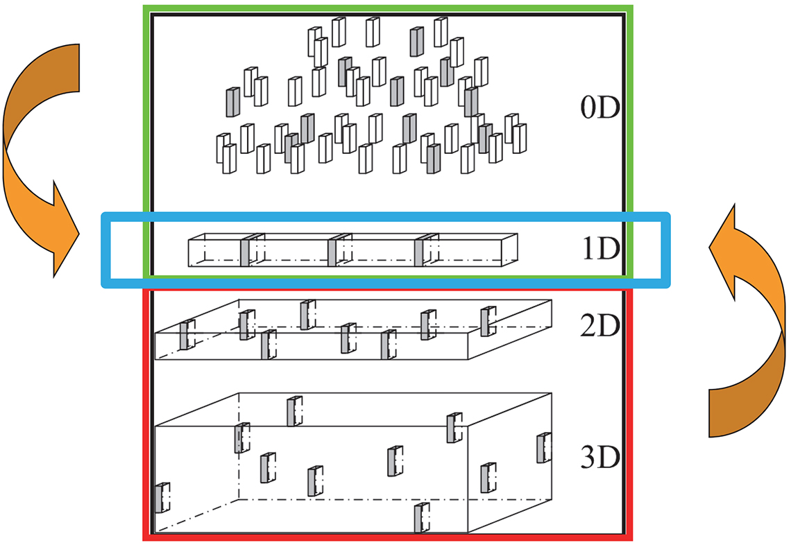
Figure 3. In practical sampling, TOS has shown the absolute desirability of transforming 3-D, 2-D and sometimes even 0-D lots into a 1-D configuration. Illustration credit: KHE.
Even if there will have to be some work involved (sometimes a lot of work) in moving, transporting (bit-by-bit) a lot, say a 3-D lot, and for example loading its content onto a conveyor belt, this is very often a welcome expenditure because of the enormous bonus(es) now available. There is no comparison because of the ease with which the gamut of sampling errors can be eliminated or reduced with the 1-D configuration. TOS’ literature is full of examples, demonstrations and case histories on this key issue, e.g. Reference 1 and literature cited herein.
The subsequent set of sampling columns will describe the full diversity of process sampling, but this is a first foray to give the reader a useful overview of what is to come.
Process sampling
Process sampling concerns 1-D lots where there is a distinct spatial (stationary lots) or temporal order between the lot units along this defining dimension. The units may appear either as an ordered series of discrete units (in time or space) or as a moving/flowing material stream. All such elongated or moving material bodies are, strictly speaking, three-dimensional objects, but by transformation into 1-D objects their sampling turns out to be identical in principle as well as in practice. The movement involved is relative: either the matter streams, or flows, past the sampler/sampling equipment, or the sampler “walks up and down” along the extended dimension of the lot. From a sampling point of view, these two situations are identical and will therefore both be covered even through the terminology most often speaks of process sampling.
It is now time to focus on the nature of the lot material to be sampled. In process sampling, the 1-D lot can be classified in three broad categories:
- A moving or stationary stream of particulate material. Examples: conveyor belts transporting aggregate materials, powders, slurries in ducts etc.
- A moving or stationary fluid flow (i.e. gasses, liquids). Examples: rivers or produced/manufactured fluids in pipelines.
- A moving or stationary stream made of discrete units. Examples: railroad cars, truck loads, or “units” (bags, drums, packages...) from a production or a manufacturing line.
Besides the distributional and constitutional heterogeneity (explained in earlier columns), there are further aspects that need to be considered to characterise the heterogeneity of 1-dimensional lots. This especially involves understanding the nature of the non-random heterogeneity fluctuations along the elongated lot. Interest is no longer so much in the heterogeneity within the units of observation (because the full slice will be extracted and its heterogeneity is therefore now only a matter for the subsequent mass-reduction step(s) which is easily managed under TOS), but specifically in the heterogeneity related to the differences between them. This is the lot heterogeneity along the entire length of the 1-D lot (which actually is the entire volume of the original lot).
Often “slicing” in such a case amounts to nothing more than appropriate selection of units viewed as a basis for a time series of analytical results. But the 1-D lot can also manifest itself as a more or less continuous body (1-, 2-, 3-phase continuum) along the length dimension, in which case it is the sampler/sampling equipment that forcefully “cuts” the stream to produce the extracted units. The location of where, and how, to cut the stream of matter is of critical importance in process sampling.
The heterogeneity contribution from an extracted unit (increment) is composed of three (four if including the total analytical error (TAE) parts in the case of 1-D processes:
- A random, discontinuous, short range fluctuation term. This term describes the constitutional heterogeneity within the increment.
- A non-random, continuous, long-range fluctuation that describes trend in the process/lot (between units) over time/distance.
- A non-random, continuous, cyclic term, describing cyclic or periodic behaviour of the process/lot.
- A random fluctuation term, taking into account all errors stemming from extraction, weighing, processing and analysis. This can be viewed as the extended TAE. Sometimes it is desired to keep the strict analytical errors isolated, as TAE proper. Either way, no confusion need arise and various cases will be illustrated in the following columns.
1-D lot heterogeneity
Characterisation of the heterogeneity of a 1-D lot must include information on the chronological order of the units extracted and their in-between correlations. Upon reflection, it is clear that it will be of interest to be able to characterise the intrinsic heterogeneity of the 1-D lot at all scales from the increment dimensions itself (there can be no resolution of the 1-D heterogeneity smaller than the physical dimension of the increment in the extension direction, which below is defined as the lag) … up to, say half the length of the entire 1-D body (corresponding to the, in practice, unlikely case in which the lot was sampled as but two very large samples, each of the magnitude of half the lot; this scale is of no practical interest in the overwhelming number of meso- and macroscopic cases, but is occasionally brought to bear on exceptionally small lots). It is actually necessary to be able to express the 1-D lot heterogeneity at all these scales simultaneously. This may appear as a complex task, but TOS has developed an amazing, and amazingly easy to derive, facility for exactly this purpose—the variogram.
Variographic analysis: a first brief
In order to characterise the autocorrelation between units of the process/lot, the variogram is very powerful. It allows understanding the variation observed between extracted increments as a function of the distance between them (in time or space). The smallest equidistance between increments to be extracted is called the “lag”. This lag is determined by the sampler when setting up the basis for a variographic characterisation (the variographic data analyst) if there has been made no variogram earlier. In certain cases valuable information from an earlier attempt will allow an optimal lag to be fixed; more on setting the critical parameter lag later. In addition, a variogram also yields information in the forms of the so-called “nugget effect”, the “sill” and the “range”, which are outlined below.
A variogram is based on the analytical results from a series of extracted increments, which are all mass-reduced and analysed in a proper TOS-correct manner—this is so as to suppress as much as possible sampling, mass-reduction and analytical errors, in complete agreement with the objectives regarding stationary lots. All extracted increments are in a sense treated as individual samples in the variographic context (but their status as grab samples is not a cause for worry, as shall be clear—because we have access to a lot of them covering the entire lot).
A variogram can be calculated based on a series of analytical results from a sufficient number of increments spanning the entire process interval of interest. An example could be a production process over a 24-h period, sampled every 20 min to characterise the variation, including three 8 h shifts. This would total 72 analytical results. More on how to fix an appropriate number of data from which to calculate variograms will be covered in later columns. Here, it is sufficient to state a beginner’s rule-of-thumb: no less than 60 data points (analytical results). Often also much shorter time-spans are investigated, for instance, during the filling of a number of bags from a batch (blending) process, or something much longer, like daily or seasonal variation, for periods up to an entire year or even more. In general, the variogram is supposed to characterise a salient “process interval of interest”; this is very much an interval that is intimately related to the specific process in question, but the common feature is that the process is “covered” with at least 60 increments.
The fundamental operative unit used in the variogram calculation is the lag parameter, j, describing the distance between two extracted units. Often the lag is expressed as a dimension-less, relative lag by only relating to a series of multipla of the basic minimum lag unit (more specifics later).
Below this column ends with an example of how to interpret a variogram; which is only meant to give an impression of the surprising wealth of information that can be gathered from a variographic analysis. Much more to come…
Interpretation of variograms
The practical interpretation of variograms is the most important step in a variographic analysis. The variogram level and form provide extensive information on the process variation captured (the systematics of the process heterogeneity captured). Normally, three primary types of variograms are encountered (based on TOS’ ~60 years of very wide experience):
- The increasing variogram (normal variogram shape).
- The flat variogram (no autocorrelation along the defining dimension).
- The periodic variogram (which is a superposition on either of the first two types).
These variograms are outlined in Figure 4.
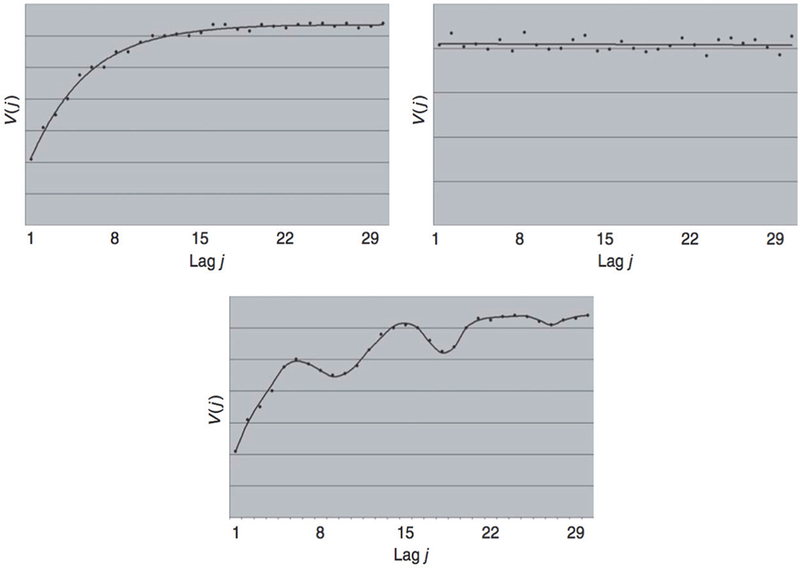
Figure 4. Three basic variogram types. Reproduced with permission from L. Petersen and K.H. Esbensen, “Representative process sampling for reliable data analysis—a tutorial”, J. Chemometr. 19, 625–647 (2005).2
When the variogram type has been identified, information on further optimisation of routine 1-D sampling can be derived (and there are many other types of information that can be gained from variograms…). The increasing variogram (Figure 4, left top variogram) can be used as an example.
Variograms are not defined for lag j = 0, as this would correspond to extracting the exact same material increment twice. Even though this is not physically possible, it is still highly valuable to acquire information as to the expected variation corresponding to if it would have been possible to repeat sampling of the exact same increment. TOS identifies this variation as the so-called “nugget effect” (also termed the “minimum possible error”, MPE). Normally, the first five points of the variogram are extrapolated backwards to intercept the ordinate axis to provide an estimate of the magnitude of the nugget effect, but there are also much more tractable model curve-fitting operators available; these are the preferential choice within geostatistics). Either way it is the estimate of the Y-axis intercept that carries a wealth of surprising information. There is a reason for the name “MPE” (minimum possible error). The nugget effect/MPE includes all error types that will be influential for sampling systems not sufficiently TOS-optimised, e.g. producing significant correct sampling errors (FSE, GSE), incorrect sampling errors as well as the TAE, all contributing to an elevated, unnecessarily inflated nugget effect. MPE is therefore an appropriate measure of the absolute minimum error that can be expected in practice using the full complement of sampling error elimination and reduction measures available in TOS. This turns out absolutely not to be the rule within very many process industry sectors—because of a desire to keep the costs of sampling systems as low as possible (which is very often too low for comfort, or rather, to put it precisely, too low to render representativity; much, much more on this aspect in many forthcoming columns).
Figure 5 shows a generic increasing variogram, delineating the three basic variogram parameters, nugget effect, range and sill, which is all that is needed to characterise any variogram.
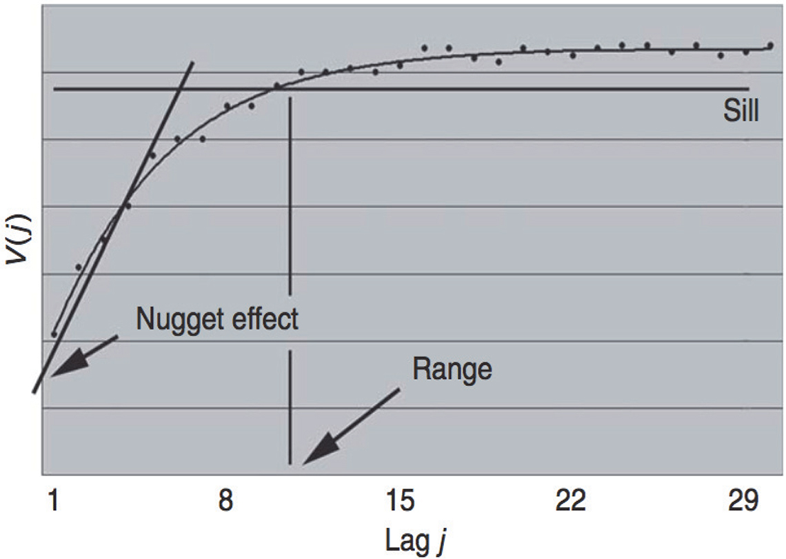
Figure 5. Generic increasing variogram, schematically defining the nugget effect, the sill and the range. Reproduced with permission from L. Petersen and K.H. Esbensen, “Representative process sampling for reliable data analysis—a tutorial”, J. Chemometr. 19, 625–647 (2005).2
When the increasing variogram becomes more or less flat after a certain multiplum of unit lags (X-axis), the “sill” of the variogram has been reached. The sill provides information on the expected maximum sampling variation if the existing autocorrelation is not taken into account. The “range” of the variogram is found as the lag beyond which there is no autocorrelation. N.B. the “dip” of a smoothed version of the variogram signifies an increase of within-unit autocorrelation as the lag becomes smaller and smaller (classical definition of time-series autocorrelation). TOS process sampling is extremely interested in what takes place with the range, i.e. in what characterises pairs of increments with a smaller between-unit distance than the range, to be more fully developed in later columns.
If a significant periodicity is observed (e.g. Figure 4, lower variogram), the sampling frequency must never be similar, since this risks introducing an additional error, an in-phase error). In these cases the specific sampling mode (random sampling, systematic sampling and stratified random sampling) becomes critically important, which is also explained in a practical application example later.
A complete introduction to variographic characterisation and process sampling is no small matter, and the present initiation will be complemented by a substantial instalment of more columns.
To whet the reader’s appetite, Figure 6.
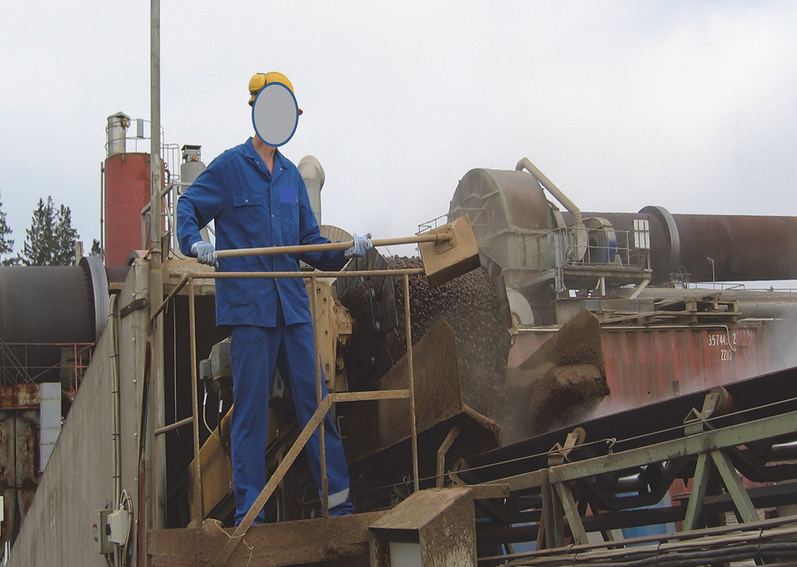
Figure 6. Manual increment extraction from a conveyor belt defining a dynamic 1-D lot. The scoop used to extract increments is less than half the width of the conveyor belt, imparting significant incorrect sampling error effects to the process sampling. This results in an (unnecessarily) inflated nugget effect, which is one of the means by which variographic process characterisation can also be used for total sampling-plus-analysis system evaluation, see, e.g., References 1 and 3. Photo credit: KHE
And for the avid and impatient reader, a recent, complete introduction to variographics can be found in Reference 4.
References
- K.H. Esbensen (Chairman Taskforce F-205 2010–2013), DS 3077. Representative Sampling—Horizontal Standard. Danish Standards (2013). http://www.ds.dk
- L. Petersen and K.H. Esbensen, “Representative process sampling for reliable data analysis—a tutorial”, J. Chemometr. 19, 625–647 (2005). https://doi.org/10.1002/cem.968
- K.H. Esbensen and P. Mortensen, “Process Sampling (Theory of Sampling, TOS) – the Missing Link in Process Analytical Technology (PAT)”, in Process Analytical Technology, 2nd Edn, Ed by K.A. Bakeev. Wiley, pp. 37–80 (2010). https://doi.org/10.1002/9780470689592.ch3
- R. Minnitt and K. Esbensen, “Pierre Gy’s development of the Theory of Sampling: a retrospective summary with a didactic tutorial on quantitative sampling of one-dimensional lots”, TOS forum 7, 7–19 (2017). https://doi.org/10.1255/tosf.96