A.M.C. Daviesa and Tom Fearnb
aNorwich Near Infrared Consultancy, 10 Aspen Way, Cringleford, Norwich NR4 6UA, UK. E-mail: [email protected]
bDepartment of Statistical Science, University College London, Gower Street, London WC1E 6BT, UK. E-mail: [email protected]
Introduction
A popular saying is “Learn to walk before you run”. We could expand this to “Learn to crawl before you learn to walk before you learn to run before you learn to sprint”. When it comes to regression analysis we have to admit that this column has spent rather more time on Partial Least Squares (PLS) than on Principal Component Analysis Regression (PCR) than on Multiple Linear Regression (MLR) and none on Classical Least Squares (CLS). This can be viewed as the opposite of the accepted wisdom of doing the easiest things first! This edition of the column is a partial redress of the admitted bias but also an explanation of why CLS is not often used in spectroscopy. Some years ago1 an attempt was made to show the relationships of the first three of these methods which more recent followers of the column might like to read. The advantages and limitations of each method are summarised in Table 1.
Table 1. Properties of different methods of regression analysis.
Method | Principle | Advantages | Disadvantages |
CLS | Addition of component spectra | Intuitive | Restricted by requirements |
MLR | Selection of a few measured variables to form a predictive equation | Easily comprehensible; very robust when applied to a few variables | Easily over-fitted when using a large number of variables and not many samples |
PCR | Computation of principal components (sources of variability in the data) followed by MLR on the PCs | Statistically sound, well researched; PCs can often be recognised; good results | More complex to understand, limited availability of good software |
PLS | Computation of new variables as a compromise between MLR and PCR to form a predictive equation | May give better results than PCR; excellent software available | More complex than PCR to understand; requires careful validation |
There have been some recent developments in the CLS method which may make it more applicable to spectroscopic data so you may see references and wonder why we had not mentioned it.
Classical least squares
The basic idea is that if you have the spectrum of a mixture and the spectra of all the components, then you can compute the composition of the mixture. For this to work there are some important requirements: the system must be linear and additive (no interactions between the components), the component spectra must be linearly independent and, for a perfect recovery of the composition, the system must be free of noise.
The theory in pictures
Figure 1 shows the “spectra” of three components, each one with a single Gaussian peak, and the spectrum of a mixture of the three in the proportions (0.5, 0.4, 0.1). All the spectra were created mathematically. The mixture spectrum in (d) was obtained by multiplying the spectra in (a), (b) and (c) by 0.5, 0.4 and 0.1, respectively, and adding the results. If we have all these four spectra, and we may assume that (d) was generated as a mixture in exactly this way but with unknown mixing proportions, then it is possible to recover the proportions from the four spectra. Under some fairly mild conditions on the component spectra, there is one and only one set of proportions that could have given the spectrum in (d).
–(c), and a mixture of all three, (d). Copyright 2010 IM Publications LLP; reproduced with permission from NIR news 21(7), 16 (2010).")
The mathematics
If we write the four spectra as column vectors of length q = 100, with s1, s2 and s3 being the pure spectra and x the mixture spectrum, then the mixing corresponds to
x = c1·s1 + c2·s2 + c3·s3 (1)
where the scalars c1, c2 and c3 are the proportions of components 1, 2 and 3 in the mixture.
Equation 1 has a matrix version. [Readers who are not conversant with matrix algebra might like to read our mini series on matrix algebra in earlier TD columns2,3,4,5,6,7 which are available on the Spectroscopy Europe website.] If we make up the 100 × 3 matrix S = [s1 s2 s3] by putting the three pure component spectra together, and the 3 × 1 vector c = [c1 c2 c3]T by putting the three proportions together, then Equation 1 can be written
x = Sc (2)
We know x and S here, and want to solve for c. If we multiply on both sides by the 3 × 100 matrix (STS)–1ST, then the result is
c = (STS)–1STx (3)
For this to work, the matrix STS, which is 3 × 3, must have an inverse. The condition for this is that the three columns of S are not linearly dependent, i.e. that no two of the three pure spectra are identical, nor can we get one of the three by mixing the other two. There is no requirement that peaks should not overlap—they overlap considerably in the example, to the extent that we only see two peaks in the mixture—merely that each pair of pure spectra must differ somewhere.
In fact we do not need the entire spectrum for this calculation. The spectra can be reduced to three spectral points, so long as the three reduced spectra still satisfy the condition of having no linear dependence between them. The tops of the three peaks would be fine, but so would most other choices that avoided the baseline.
The noisy case
If the system behaves as assumed, and there is no noise anywhere, Equation (3) recovers the exact proportions in the mixture. This is a calculation, not an estimation. Alas, real systems have noise. Suppose we assume additive independent noise, so that Equation (1) becomes
x = Sc + e
This is the familiar linear model, with c playing the role of parameter vector, and Equation (3) is the equally familiar least squares estimate of c. Thus the formula does not change when we have a noisy system, but the result is now an estimate of the proportions in the mixture and not an exact calculation.
How good an estimate it is will depend on the amount of noise, and also on how distinct are the three pure spectra. The overlap between the peaks in (a) and (b) did not matter when there was no noise, but when there is noise this overlap will degrade the quality of the estimates to some extent. What happens in the matrix algebra is that the off-diagonal terms in STS get larger as the correlations between the pure spectra increase. This makes the inverse less well-conditioned, which in turn multiplies the noise up by larger factors in the calculations of Equation (3).
Now it is worth having more than three spectral points, since the surplus information is essentially averaged in the estimation procedure, reducing the noise in the result. Cutting off the spectra at about point 70 might just be worth it though: the flat baseline will only contribute its noise, and although the contribution will be small one might as well remove it.
The drawbacks
The reason this approach is rarely used in spectroscopy is that the assumptions of linearity and additivity are almost never satisfied, despite the habitual citation of Beer’s Law (especially in papers on NIR spectroscopy!). There is also the requirement that the spectra of the pure components be known. Interestingly, this need not involve measuring spectra on the pure components themselves. The pure spectra can be inferred from measurements on a suitable set of mixtures with known proportions using the same sorts of ideas as those described above, but working the other way round. Unfortunately in many applications we are not even sure how many components there are in our mixture, let alone what their spectra might be. When working in reflectance mode, scatter effects are also a problem since the introduction of arbitrary multiplicative factors into all the spectra rather spoils the maths.
For all these reasons, this approach in its simple form as presented above is not often useful for spectroscopy. So when colleagues ask you “Why don’t you use CLS?” you now know the answer! However, it can provide a starting point for more sophisticated approaches that may be useful in the future.
Reading more
There is a very detailed description of CLS, with two worked examples, in the chemometrics book by Beebe, Pell and Seasholtz.8 It is also explained there how the method can easily be extended to cope with variable linear baselines. The paper by Mark et al.9 discusses the units for the concentrations that the mixture proportions represent (weight fraction? volume fraction? ...), something that is not important for the mathematics but is important in a real example and this needs to be taken seriously if you think that you have an example that fulfils the requirements.
Acknowledgement
The majority of this column is reproduced from a “Chemometric Space” article by Tom published in NIR news10 and we are grateful to IM Publications for permitting us to re-use it.—Tony
References
- A.M.C. Davies and T. Fearn, “Back to basics: observing PLS“, Spectroscopy Europe 17(6), 28 (2005).
- A.M.C. Davies, “The magical world of matrix algebra”, Spectroscopy Europe 12(2), 24 (2000).
- A.M.C. Davies and T. Fearn, “The TDeious way of doing Fourier transformation (Lesson 2 of matrix algebra)”, Spectroscopy Europe 12(4), 28 (2000).
- A.M.C. Davies and T. Fearn, “Changing scales with Fourier transformation [Lesson 3 of matrix algebra (matrix multiplication)]”, Spectroscopy Europe 12(6), 22 (2000).
- A.M.C. Davies and T. Fearn, “A very simple multivariate calibration [Lesson 4 of matrix algebra (matrix inversion)]”, Spectroscopy Europe 13(4), 16 (2001).
- A.M.C. Davies and T. Fearn, “Vectorisation in Matrix Algebra [Lesson 5 of Matrix Algebra (Vectorisation)]”, Spectroscopy Europe 13(6), 22 (2001).
- A.M.C. Davies and T. Fearn, “Doing it faster and smarter (Lesson 6 of Matrix Algebra)”, Spectroscopy Europe 14(6), 24 (2002).
- K. Beebe, R.J. Pell, M.B. Seasholtz, Chemometrics: a Practical Guide. Wiley, New York (1998).
- H. Mark, R. Rubinowitz, D. Heaps, P. Gemperline, D. Dahm and K. Dahm, Appl. Spectrosc. 64(9), 995 (2010).https://doi.org/10.1366/000370210792434314
- T. Fearn, “Classical least squares”, NIR news 21(7), 16 (2010).