Karl H. Norrisa with A.M.C. Daviesb
aConsultant, 11204 Montgomery Road, Beltsville, MD 20702, USA
bNorwich Near Infrared Consultancy, 10 Aspen Way, Cringleford, Norwich NR4 6UA, UK. E-mail: [email protected]
Introduction
I expect that many of you will have recognised the name of Karl H. Norris as the man the Near Infrared community calls “The father of NIR spectroscopy”. Karl celebrated his 90th birthday last May but he hasn’t stopped thinking and working. When he told me the subject of his recent EAS lecture I asked him if he would contribute a column, as it was fortuitously so compatible with my previous columns on looking at spectra.1,2 He agreed, but in fact it will be two columns. In this first one he introduces his calculation method for fourth derivatives and shows how it can be used to extract instrument noise. The second column will look at sample temperature effects, and viewing the effects of changes in the composition of samples.—Tony Davies
Formula for computing second derivative:
\[f''(x) = \mathop {\lim }\limits_{h \to 0} \frac{{f(x + h) - 2f(x) + f(x - h)}}{{{h^2}}}\]
Note that (h) must be greater than zero. The size of the gap (h) has a very useful effect on the derivative.
We define the fourth derivative spectrum as the second derivative of a second derivative spectrum.
We have tested three different computer programs for computing the fourth derivative of an NIR spectrum and the result is different for each.
- A computer program developed by K. Norris, in Lab-Calc™ which uses the above formula.
- Vision software from Foss NIRSystems which includes a segment and does not divide by the square of (h).
- Unscrambler 9.8 from Camo which allows a Gap choice such that
h = Gap + 1
Calculation of fourth derivative
Like Tony, I also like to look at spectra in great detail, and I have been searching for the best tool for such observations. I have decided that the fourth derivative with different gap sizes is the best.3
However, to understand fourth derivative spectra I suggest starting with computer-generated spectra with defined bandwidths and amplitudes to learn what the fourth derivative does to spectra.
Figure 1 shows four spectra with bandwidths of 2 nm, 10 nm, 20 nm and 100 nm, plus a random noise spectrum to simulate instrument noise.

The sum of these five spectra is shown in the same figure. Please note that the 100 nm spectrum has been divided by 20 for plotting.


Figure 2 shows the spectrum extracted from the five-sum spectrum with a fourth derivative using Unscrambler 9.8 with a gap of one. This small gap derivative shows the 2 nm absorber and the random noise. The other bands are not detected. Figure 3 shows the 10 nm band, the 2 nm band and the 20 nm band with smaller random noise for a fourth derivative with a gap of nine. The 100 nm band is not detected. Figure 4 shows the 10 nm band, the 2 nm band, the 20 nm band and a distorted 100 nm band along with a reduced noise signal for fourth derivative with a gap of 19. Figure 5 shows the result for a fourth derivative with a gap of 96; Unscrambler 9.8 would not use a gap value greater than 96. Here we observe a good representation of the original spectrum of Figure 1.
The random noise spectrum is shown in Figure 6, along with the spectrum obtained with a fourth derivative gap of two and ten. The noise gets rescaled, because of the division by h2 in the derivative calculation.

Now let me use the fourth derivative on real NIR spectra. Figure 7 shows nine repeated scans of one finely ground wheat sample as measured in the reflection mode with an NIRSystems model 6500. The sample is contained in a rotating sample cell, and in this experiment the reference standard was measured, the sample was inserted into the instrument, and remained in the instrument for the subsequent scans. After three scans were recorded, a cup of coffee was placed at the back of the instrument near the air filter. Three more scans were recorded, and the cup was removed for the final three scans.

The purpose of the experiment was to determine if the humidity in the instrument could be changed by adding the hot cup of coffee, and could the change be observed on the recorded spectra. Figure 7 shows no evidence of any change in the spectra, but if we subtract the spectrum of sample #1 from sample #5, and compute the fourth derivative with a gap of four, a large change in spectra can be observed (Figure 8). We observe typical instrument noise in the region below 800 nm and above 2000 nm, but we also see many narrow-band peaks in the 1350 nm and 1860 nm regions from the change in humidity. The same fourth derivative applied to the difference of #1 from #3 shows slight evidence of a change in humidity before the coffee cup was placed near the instrument. Please note that the atmospheric bands of water have a band-pass of less than 2 nm, but the instrument with a spectral resolution of 10 nm converts the atmospheric bands to 10 nm bands. The fourth derivative treatment also shows definite noise peaks in the 1100 nm region. This noise in common on this instrument model, because the instrument incorporates two different monochromators into the instrument. One monochromator covers the spectral region from 400 nm to 1100 nm, and the second covers the spectral region from 1100 nm to 2500 nm. The instrument incorporates correction based on a reflection standard to fit the two spectra together, but this correction may not be adequate for sample scans. This error can be seen in the Log(1/R) plot in Figure 7.

Now a look at ten beautiful scans of a polystyrene window with an FT-NIR instrument recorded with 4 cm–1 resolution (Figure 9). Many clearly defined absorption bands are evident. Note the data have been converted to a wavelength scale. Figure 10 shows the spectrum from one of the scans, along with fourth derivative treatment with a gap of two and a gap of ten. The fourth derivative spectra have been multiplied by large numbers for plotting on the same chart as the Log(1/T) spectrum of the sample. This shows the advantage of changing the gap to emphasise narrow-band absorbers, as well as showing the bands inherent in the sample. Again we observe atmospheric bands in the sample spectrum with a gap of two, but now we see many more bands, because this instrument has a spectral resolution of about 2 nm in the 1860 nm region. The instrument was adequately purged for measuring the polystyrene sample, because the polystyrene bands did not occur in the regions where the atmospheric bands occur. The polystyrene bands in the 2160 nm region are badly distorted using a fourth derivative gap of two, but the gap of 10 shows the polystyrene bands. To examine the polystyrene bands more thoroughly a fourth derivative with a gap of four was applied. This provided a spectrum containing instrument noise, so a smoothing routine was applied to minimise the noise. This author prefers the Gaussian routine for smoothing of spectra, but when a Gaussian smooth with five points was applied in Unscrambler 9.8 it appeared the peaks had been shifted in wavelength. Therefore, a Savitsky–Golay with five points was applied in place of the Gaussian smooth.


Figure 11 shows the Log(1/R) spectrum of the polystyrene along with the fourth derivative at a gap of four and the two smoothing curves. We now observe that there are at least eight absorption bands in this polystyrene sample in the 2160 nm region. The wavelength shift is obvious, and the Gaussian smoothing function in Unscrambler 9.8 is in error. A quick test with version 10.1 showed that it agrees with the Savitsky–Golay results.

Conclusion
These are just a few of many tests in using the fourth derivative to allow a better understanding of NIR spectra. In the second part we will see how the fourth derivative can be used to emphasise spectral variations caused by temperature changes and changes in sample composition.
References
- A.M.C. Davies, Spectroscopy Europe 23(2), 24 (2011).
- A.M.C. Davies, Spectroscopy Europe 23(4), 24 (2011).
- T. O’Haver, An Introduction to Signal Processing in Chemical Analysis, http://terpconnect.umd.edu/~toh/spectrum/TOC.html. Accessed 29 November 2011. (A very useful introduction to the subject of digital signal processing—TD.)