A.M.C. Davies
Norwich Near Infrared Consultancy, 10 Aspen Way, Cringleford, Norwich NR4 6UA, UK. E-mail: [email protected]
Introduction
I have been thinking that it is about time (or it will be soon) that I should retire from producing my share of the Tony Davies column. “Going the last mile” is a familiar term and a furlong (a very old English measure of distance) is 1/8th of a mile. I am not sure how many furlongs there will be, but they will be a review of the chemometric ideas that have most excited me over the last 30 years. The furlong is the classic measure of distance in horse racing so irrespective of the distance; the race ends with the “last furlong”. There will be a last furlong for these columns. Please note that the furlong is a fundamental unit in the FFF (furlong/firkin/fortnight) system!1
Chemometrics of data compression
One of the most important ideas in chemometrics is data compression. This is the reduction in the number of variables without the loss of information. Compression may be applied to a data set (spectra of different samples) or to an individual sample (a spectrum).
Spectroscopy usually provides spectra of samples with data for a large number of variables (wavenumbers or wave lengths). When I started in NIR spectroscopy we had spectra with 700 data points. The first chemometric method we used was multiple regression analysis and there were far too many variables. My friend Ian Cowe began to use principal component analysis (PCA) to reduce the number of variables, but I could not copy him because the only PCA program available to me was limited to a maximum of 100 variables. In 1982 I went to the first IDRC at Chambersburg where I met Professor Fred McClure. Fred introduced me and the meeting to the use of Fourier Transformation (FT) for compressing spectral data.2 The idea did not seem to impress many delegates, but I was very excited by it because I immediately realised that this was the way to fit my spectra into PCA. It was my entry point to chemometrics and a long collaboration with Fred McClure.
Data compression by Fourier Transformation
Fourier transformation (FT) involves the addition of series of sine and cosine waves, and the mathematics of what we now call “Fourier Transformation” were invented by the French physicist Joseph Fourier to help him in his work on the propagation of heat in 1807.2 FT is complex and requires extensive calculations. Early computers were too small and much too slow to be used for FT! The speed problem was much reduced with the invention and publication of the Fast Fourier Transformation (FFT) by Cooley and Tukey3 in 1965.
Summing sine waves
In order to keep things as simple as possible we are just going to sum sine waves but I am sure you can imagine that with the extra addition of cosines the effects are similar but more complex.
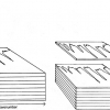
The top half of Figure 1 shows two sine waves, one of one cycle and the other of three cycles. It is not difficult to imagine that the addition of these two waves will produce the slightly more complex wave in the lower part of Figure 1. The top half of Figure 2 shows a series of sine waves with odd numbers of cycles from 1 to 15. What would be the sum of these eight waves? The answer is shown in the lower part of the Figure. It is not difficult to see that if we extended the number of sine waves then the sum would approach the shape of a square wave as shown in Figure 3.


If we can go from a sine wave to a square wave just by adding sine waves is there any limit to what shape we can fit? In 1807 Joseph Fourier proposed that any curve could be fitted by the summation of a series of sine and cosine waves. Now that we have the added benefit of the FFT these can be readily computed on even a low specification PC. The output from the program is a series of “a” and “b” coefficients for the series of sine and cosine waves.
Applying FT to NIR spectra
Figure 4 is an NIR spectrum of a PET plastic recorded at 2 nm intervals over the range 1100–2498 nm, so we have 700 wavelength values. The spectrum is typical of many NIR spectra in that there is an upward trend. This would cause a problem with the FT because the mathematics assumes that the waveform repeats to infinity in both directions; if the ends are not equal then the discontinuity will give rise to a series of high frequency oscillations known as “ringing” at each end of the spectrum. This irritation can be readily removed by calculating a tilt and removing this from each point in the spectrum. The lower spectrum in Figure 4 is the result of this procedure.
 and tilted (blue) NIR spectrum of a sample of PET.")
If we have 700 wavelengths, we will compute 350 pairs of Fourier coefficients and these are shown for the (tilted) spectrum of the PET spectrum as 350 “a” coefficients followed by 350 “b” coefficients in Figure 5.

An important point, which may be obvious but I need to stress it, is that this process is exactly reversible. Figures 4 and 5 are two views of the same information, if we have one we can calculate the other but, of course, we have not yet achieved any data compression.
FT data compression
A few of the coefficients shown in Figure 5 are larger than the majority, while many of the majority are close to zero and this makes it possible to reduce (i.e. compress) the data by not saving these very small coefficients. It is often found that, as in Figure 5, most of the useful information in the frequency domain is found at low to moderate frequencies and the high frequencies can be ignored. The higher frequencies are just forgotten during data storage, transmission or processing and are replaced by zeros when reconstructing the original spectrum. The difference between the original and a well-reconstructed spectrum is often seen to be noise and thus the FT process can achieve data compression and high frequency noise reduction in the single operation.
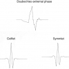
The effects of saving only 20 pairs or 100 pairs of coefficients on the reconstruction of the spectrum are shown in Figures 6 and 7, respectively. The green line at the bottom of the figure is the difference between the original (black) spectrum and the (red) reconstruction. With only 20 pairs of Fourier coefficients the error is obvious, but with 100 coefficients it is almost a straight horizontal line. The line is plotted on its own scale in Figure 8 and it can be seen that this is characteristic of high frequency noise and can be advantageously removed.
, reconstructed (red), tilted (blue) and difference (green) spectra using 20 pairs of Fourier coefficients for the reconstruction of the spectrum in Figure 5.")


Thus we can see that for this spectrum we can reduce the size of the spectrum file by 70% while at the same time removing some high frequency noise but not losing information.
Some further mathematics?
If you are interested in understanding the mathematics more completely, Tom Fearn and I have previously published two columns4,5 in our mini-series on matrix algebra using FT as an example. You can find them on the Spectroscopy Europe website.
In the next “furlong” we will discuss a more recent method of data compression, wavelets.
References
- Stan Kelly-Bootle, “As big as a barn?”, ACM Queue 62–64 (March 2007). http://queue.acm.org/detail.cfm?id=1229919
- F.G. Giesbrecht, W.F. McClure and A. Hamid, Appl. Spectrosc. 35, 210 (1981). doi: 10.1366/0003702814731590
- J.W. Cooley and J.W. Tukey, “An algorithm for the machine calculation of complex Fourier series”, Math. Comput. 19, 297–301 (1965). doi: 10.2307/2003354
- A.M.C. Davies and T. Fearn, “The TDeious way of doing Fourier transformation (Lesson 2 of matrix algebra)”, Spectrosc. Europe 12(4), 28 (2000). http://bit.ly/Ze6VFV
- A.M.C. Davies and T. Fearn, “Changing scales with Fourier transformation [Lesson 3 of matrix algebra. (Matrix multiplication)]”, Spectrosc. Europe 12(6), 22 (2000). http://bit.ly/Zlr2io