A.M.C. Davies
Norwich Near Infrared Consultancy, 75 Intwood Road, Cringleford, Norwich, NR4 6AA, UK
Partial least squares (PLS) was invented by Herman Wold in the 1970s1 and then modified by his son Svante and Harald Martens in the early 1980s2 for use in regression. However, as anyone who has been reading these columns or taking a general interest in chemometrics will know, the name that is most strongly associated with partial least squares (regression) (PLS) is Harald Martens’. PLS is, of course, widely used by the NIR and chemometric communities but Harald has been irritated for many years by the reluctance of the statistical community to accept it. One of the criticisms of PLS has been the lack of established statistical theory for significance testing of the model parameters. Last year Harald and his wife Magni published3 a very clever way of achieving not only a test but (with Frank Westad) of using it as a method of selecting those variables that should be retained in a PLS regession.4,5 I am able to demonstrate it for you as the procedure has been included into the latest version (7.6) of the Unscrambler® software package from Camo. The method was first called “The Jacknife” but this terminology has been used elsewhere in statistics so it may be better to call it “Uncertainty testing”. This is the name used by Camo.
Uncertainty testing
We often use cross-validation6 in the development of PLS methods to determine the number of factors which should be retained. When the original programs were written, computer memory was at a premium and so only intermediate results that were required later could be retained. Nowadays, we are generally rich in storage space and so we can retain as many intermediate calculations as we like. When we do cross-validation by the original program it does not retain all the estimates of the regression coefficients but the Martenses realised that if you did, then you could use them to estimate the variance of the coefficients and hence test if they were significantly different from zero. Once you have the test you can then proceed to use it to decide which variables should be dropped from the original data set.
A demonstration
I am continuing to use the Camo octane data set7 mainly because I can refer to previous articles,8,9 which hopefully some of you will remember! It is not supposed to be an ideal set for such a demonstration. The set contains a training set of 26 and a test set of 13 samples measured at 226 NIR wavelengths with octane number measurements as the reference chemistry.
The last time I used the data I showed that after we had eliminated two outlying samples we could develop a PLS regression that gave a RMSEP of 0.41. Another possible calibration based on the first 101 variables did not perform well on the test set and gave a RMSEP of 0.88.
Figure 1 shows the calibration plots for the model using all variables but omitting the two outliers. This used full cross-validation (i.e. every sample in turn was left out, a model was computed and used to predict that sample) but I also ticked the new “Uncertainty test” box. Figure 2 shows the regression coefficients with the significant variables marked. These indicate two areas of the data with significant coefficients. From the previous study9 we know that the second area is associated with the outliers so it will be a good idea to use the first area. Figure 3 shows the results of building a new model with this reduced set of 40 variables. As this was a new model I included all the data, and the scores plot (top left) does not indicate the presence of any serious outliers so we can use all 26 samples in the training set. When tested on the 13 samples in the test set, this model gives a RMSEP of 0.33 this appears to be an improvement but we are not finished yet. I had again ticked the “Uncertainty test” box so that we can see if all the variables in the reduced set give rise to significant coefficients. The plot, Figure 4, shows that only eighteen of them are significant so we go round the loop again and compute a model with these eighteen variables; the results are shown in Figure 5. This model gives a RMSEP on the test set of 0.31, Figure 6. It is unlikely that this result is significantly different from the 40 variable model but if it had been tested on a reasonably large data set it would be preferred because the model contains fewer terms.
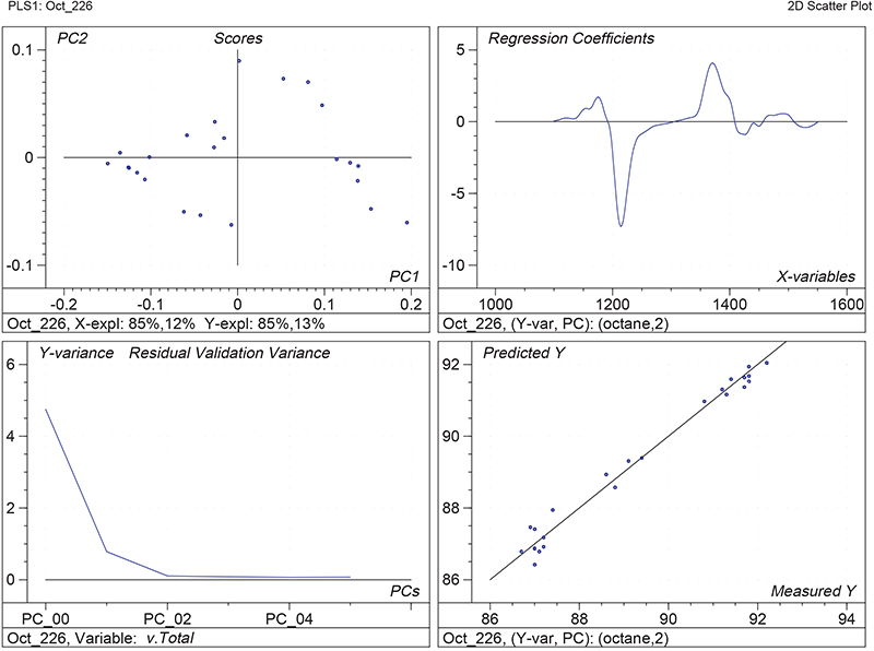
Figure 1. Calibration for octane using 226 NIR variables. Clockwise from top left: scores plot for first two factors; regression coefficients against wavelength; predicted against reference for the calibration set; residual validation variance against number of factors (PCs in Camo terminology).
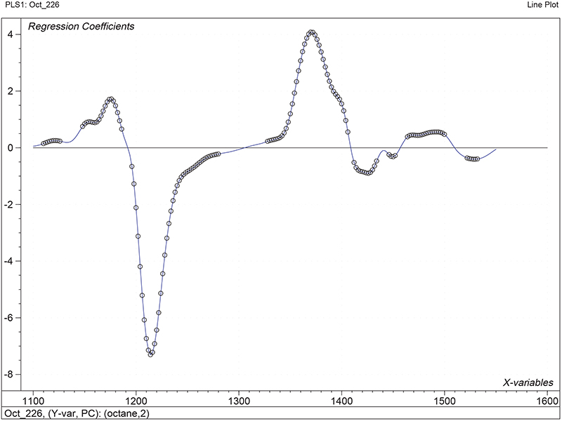
Figure 2. Significant regression coefficients in the regression shown in Figure 1.
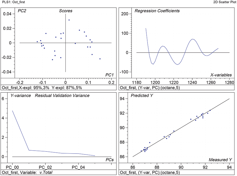
Figure 3. Calibration for octane using 40 NIR variables. Plots as Figure 1.
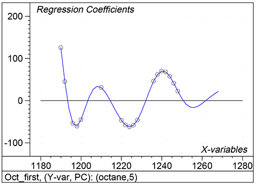
Figure 4. Significant regression coefficients in the regression shown in Figure 3.
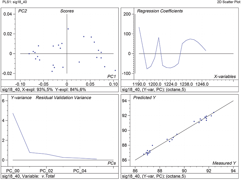
Figure 5. Calibration for octane using 18 NIR variables. Plots as Figure 1.
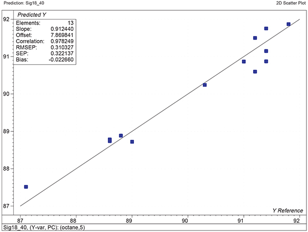
Figure 6. Plot of predicted against reference for the test set using the calibration shown in Figure 5.
There are some additional benefits that come from uncertainty testing and one of these is shown in Figure 7. This shows the variability of the factor scores from each iteration of each sample in the cross-validation. The centre of each “star” is the final model, while the results from each iteration are shown as a cross with a line to the centre. The circle indicates the computed score when that sample was left out of PLS calculation. If it is far from the centre (sample 26) then it indicates that it is a sample with high influence.
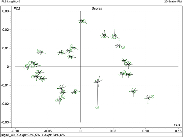
Figure 7. Stability scores plot for the first two factors of the calibration shown in Figure 5.
Uncertainty testing is a “win-win” development for PLS. Not only has Harald been able to provide an important test for the regression coefficients but the test provides us with a simple method of reducing the number of unnecessary variables, which should give rise to more robust models that are also more easily transferred across different spectrometers. As Westad and Martens have shown, it is not very difficult to automate the procedure so in the future I think we will see PLS calibrations which utilise relatively few variables become the norm.
Anyone who is interested in understanding the underlying statistics should read the description of “The Jacknife” by Tom Fearn.10
References
- H. Wold, “Soft Modelling by Latent Variables: The Partial Least Squares Approach”, in Perspectives in Probablity and Statistics, Ed by J. Gani. Academic Press, London (1975).
- S. Wold, H. Martens and H. Wold, in Proceedings of the Conference on Matrix Pencils, March 1982. Lecture Notes in Mathematics, Ed by A. Ruhe and B. Kågstrom. Springer Verlag, Heidelberg, pp. 286–293 (1983). https://doi.org/10.1007/BFb0062108
- H. Martens and M. Martens, Food Quality and Preferences 10, 233 (2000). https://doi.org/10.1016/S0950-3293(99)00024-5
- F. Westad, M. Byström and H. Martens, in Near Infrared Spectroscopy: Proceedings of the 9th International Conference, Ed by A.M.C. Davies and R. Giangiacomo. NIR Publications, Chichester, pp. 247–251 (2000). https://www.impopen.com/fbooks-toc/978-1-906715-21-2
- F. Westad and H. Martens, J. Near Infrared Spectrosc. 8, 117 (2000). https://doi.org/10.1255/jnirs.271
- A.M.C. Davies, Spectroscopy Europe 10(2), 24 (1998).
- Available from the Camo website: www.camo.no/.
- A.M.C. Davies, Spectroscopy Europe 10(4), 28 (1998).
- A.M.C. Davies, Spectroscopy Europe 10(6), 20 (1998).
- T. Fearn, NIR news 11(5), 7 (2000). https://doi.org/10.1255/nirn.580